TL;DR: I'm analyzing gene expression data from 40 human participants in a diet study, comparing control vs. "special" diets at 3 timepoints (baseline, 4 weeks, 12 weeks). Most of my differential expression results seem unusual, especially with more significant changes in the control group than expected. I've run several comparisons, but results are inconsistent. Any suggestions on troubleshooting, improving the analysis, or accounting for baseline gene expression?

Hi Michael,

Apologies if this has already been addressed, but I could really use some guidance. I'm also extremely new to all of this so sorry if some of this is already widely known!

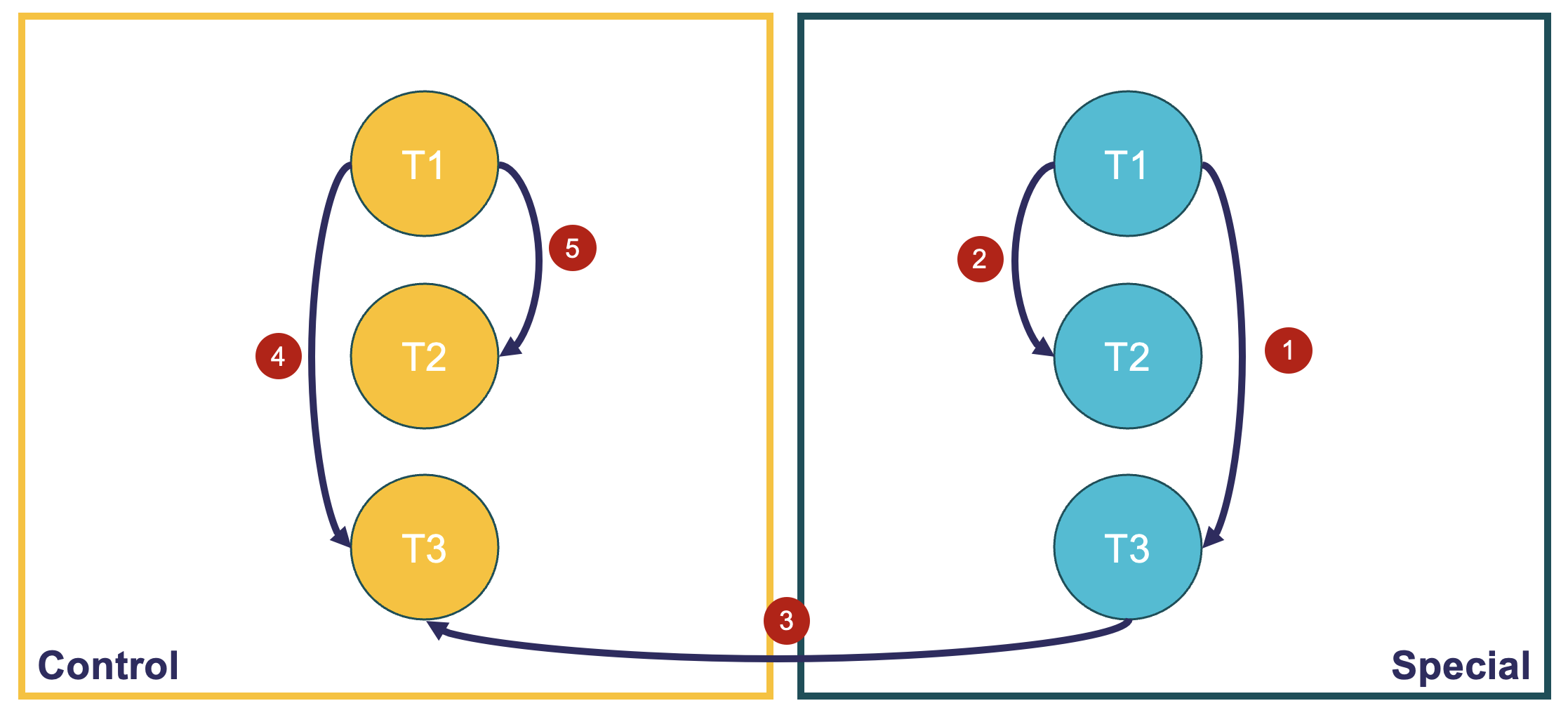
Background: I have data from 40 human participants, randomly assigned to one of two groups (~20 in each): control diet and "special" diet. Samples were collected at 3 timepoints (baseline, 4 weeks and 12 weeks). I'm trying to see whether gene expression has changed in response to the diet. These are the comparisons (see image 1) I would like to make:

RStudio Analysis: Here is an example of how I ran one of the comparisons (n1) in RStudio:

sampleinfo<-read.csv("samplesheet.csv")
sampleinfo <- sampleinfo %>%
  filter(!(Group == "Control" | Timepoint == "T2")) 

files<-file.path("salmon_outputs", sampleinfo$participant_ID, "quant.sf") #here change "salmon_outputs" to your directory name
files<-set_names(files, sampleinfo$participant_ID)

#to make txi object 
tx2gene <- read_tsv("tx2gene.tsv") 

  txi <- tximport(files, type = "salmon", 
                  tx2gene = tx2gene, 
                  ignoreTxVersion = TRUE,
                  countsFromAbundance = "lengthScaledTPM")

  ###save for future use 
  saveRDS(txi, file = "txi_lowsug_t1_vs_t3.rds")}

#txi<-readRDS("txi_lowsug_t1_vs_t3.rds")

all(colnames(txi$counts)==sampleinfo$participant_ID) #check this matches

#make a model that "predicts" gene expression. make it as simple as possible 
sampleinfo$Timepoint <- factor(sampleinfo$Timepoint, levels = c("T1", "T3")) #just to make sure T1 is first
simple.model<- as.formula(~ Timepoint)
#model.matrix(simple.model, data = sampleinfo)

ddsObj.raw <- DESeqDataSetFromTximport(txi = txi,
                                       colData = sampleinfo,
                                       design = simple.model)

keep <- rowSums(counts(ddsObj.raw)) > 20
table(keep, useNA="always")
ddsObj.filt <- ddsObj.raw[keep, ]
ddsObj<-estimateSizeFactors(ddsObj.filt)

logcounts<-log2(counts(ddsObj, normalized = FALSE) + 1)
logNormCounts<-log2(counts(ddsObj, normalized = TRUE) + 1)

#library(limma)
limma::plotMA(logcounts, array = 5)
abline(h = 0, col = "red")
limma::plotMA(logNormCounts, array = 5)
abline(h = 0, col = "red")

## estimating dispersion
ddsObj_test<-estimateDispersions(ddsObj)
plotDispEsts(ddsObj_test)
ddsObj_test<-nbinomWaldTest(ddsObj_test)
results.simple<-results(ddsObj_test, alpha = 0.05)

#upregulated
sum(results.simple$log2FoldChange > 0 & 
      results.simple$padj <0.05, na.rm = TRUE)
#65 genes

#downregulated
sum(results.simple$log2FoldChange < 0 & 
      results.simple$padj < 0.05, na.rm = TRUE)
#94 genes
hist(results.simple$pvalue)

# include your problematic code here with any corresponding output 
# please also include the results of running the following in an R session 

sessionInfo( )
R version 4.4.3 (2025-02-28)
Platform: aarch64-apple-darwin20
Running under: macOS Sequoia 15.3.2

Matrix products: default
BLAS:   /System/Library/Frameworks/Accelerate.framework/Versions/A/Frameworks/vecLib.framework/Versions/A/libBLAS.dylib 
LAPACK: /Library/Frameworks/R.framework/Versions/4.4-arm64/Resources/lib/libRlapack.dylib;  LAPACK version 3.12.0

locale:
[1] en_US.UTF-8/en_US.UTF-8/en_US.UTF-8/C/en_US.UTF-8/en_US.UTF-8

time zone: Europe/London
tzcode source: internal

attached base packages:
[1] stats4    stats     graphics  grDevices utils     datasets  methods   base     

other attached packages:
 [1] lubridate_1.9.4             forcats_1.0.0               stringr_1.5.1              
 [4] dplyr_1.1.4                 purrr_1.0.4                 readr_2.1.5                
 [7] tidyr_1.3.1                 tibble_3.2.1                ggplot2_3.5.1              
[10] tidyverse_2.0.0             DESeq2_1.44.0               SummarizedExperiment_1.34.0
[13] Biobase_2.64.0              MatrixGenerics_1.16.0       matrixStats_1.5.0          
[16] GenomicRanges_1.56.2        GenomeInfoDb_1.40.1         IRanges_2.38.1             
[19] S4Vectors_0.42.1            BiocGenerics_0.50.0         tximport_1.32.0            

loaded via a namespace (and not attached):
 [1] gtable_0.3.6            lattice_0.22-6          tzdb_0.5.0              vctrs_0.6.5            
 [5] tools_4.4.3             generics_0.1.3          parallel_4.4.3          pkgconfig_2.0.3        
 [9] Matrix_1.7-3            lifecycle_1.0.4         GenomeInfoDbData_1.2.12 compiler_4.4.3         
[13] munsell_0.5.1           codetools_0.2-20        pillar_1.10.1           crayon_1.5.3           
[17] BiocParallel_1.38.0     DelayedArray_0.30.1     abind_1.4-8             tidyselect_1.2.1       
[21] locfit_1.5-9.12         stringi_1.8.7           grid_4.4.3              colorspace_2.1-1       
[25] cli_3.6.4               SparseArray_1.4.8       magrittr_2.0.3          S4Arrays_1.4.1         
[29] withr_3.0.2             scales_1.3.0            UCSC.utils_1.0.0        bit64_4.6.0-1          
[33] timechange_0.3.0        XVector_0.44.0          httr_1.4.7              bit_4.6.0              
[37] hms_1.1.3               rlang_1.1.5             Rcpp_1.0.14             glue_1.8.0             
[41] rstudioapi_0.17.1       vroom_1.6.5             jsonlite_2.0.0          R6_2.6.1               
[45] zlibbioc_1.50.0

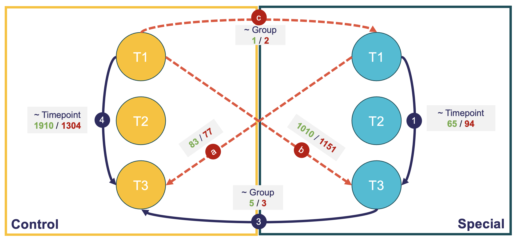
Issue: I have completed most of my comparisons, but the results seem strange. I did not expect that many more differentially expressed genes in the control group compared to the experimental group. Similarly, it then does not add up that the control and the special groups at T3 do not have that many differentially expressed genes (see analysis 3).

Note: Green denotes number of upregulated genes, and red the number of downregulated genes.

So then I ran some sensitivity comparisons (denoted by the dashed red lines) and I think this has further confused me as I was expecting really different results. I might be extremely wrong, but if the results were true and, since both groups should be the same at baseline (randomly assigned), I would expect analysis a to produce similar results to analysis 4, and analysis b to produce similar results to analysis 1.

Questions

• I'm super new to all of this: have I done something wrong?
• What would you do next to investigate what is happening?
• Since is human data and very noisy, is there a way to account for baseline gene expression for each individual? e.g. in analysis n1, could we potentially put T1 as a covariate, or subtract T1 from T3?

Thank you for your time and help!

Benny