I am currently working on giving users much more control over normalization in DiffBind. In the meantime, there is a trick you can do you avoid normalization when using DESeq2 as the analysis method.
After running dba.count(), you can change the individual library sizes to all be the same. Then if you run dba.analyze() with bFullLibrarySize=TRUE (default) the normalization facts will all be equal to 1. You probably want to run dba.analyze()with bSubControl=FALSE to avoid having the control reds subtracted if do not want normalization of any kind.
Also, there is a "backdoor" in DiffBind to allow you to provide your own normalized read counts -- if that is of interest, I can show the code required to use it.
In my opinion, for visualization purposes it's accurate enough to convert the raw reads (bam files) to tdf format and load them in IGV with the option "normalize coverage data" enabled, this will rescale the raw counts to 1000000 / total counts.thus correcting for different library sizes. This assuming you are using/willing to use IGV, other browsers surely have similar options.
DiffBind, or rather the underlying edgeR and DESeq packages, don't make use of the read profiles. All they use are the raw counts of reads in given intervals (ChipSeq peaks, genes, whatever), in fact the read profile within an interval doesn't enter in the analysis at all.
If you want to show the log fold change you could prepare a bedgraph file where each line has as coordinates the region tested, or maybe the midpoint of the region tested, whichever looks better, and as value (4th column) the log fold change. Then load this file in IGV with or without the raw reads file as above.
The recently released version of DiffBind includes a new interface function, dba.normalize(), that allows library sizes and normalization factors (or offsets) to be set and retrieved directly. The updated vignette includes a detailed exploration of the impact of different normalization schemes.
Dear author,
I have a similar question. dba.plotMA could easily generate ma plots under raw counts (bNormalized = F), but there is no way to retrieve that data behind the MA plot?
I followed your advice in specifying the same library size for my samples, and use full library size in dba.normalize() step. But I still get results in the dba.analyze step which is different from what my raw counts ma plot shows. Looks like there is some normalization going on.
If you check on the demo data tamoxifen.
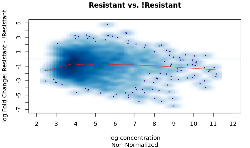
The ma plot for the raw data is:
And I run the following to run the analysis without normalization:
tamoxifen$class[8,] = 1e+07
tamoxifen = dba.normalize(tamoxifen,  normalize = DBA_NORM_LIB, library = DBA_LIBSIZE_FULL) ### at this stage the library sizes should be all the same, hence the normalization factors
tamoxifen = dba.analyze(tamoxifen, method = DBA_DESEQ2)
dba.plotMA(tamoxifen, bUsePval = F)
And the ma plot is now:
I appreciate your suggestions as why there is still some sort of "normalization" in my attempt to suppress normalization.


 And I run the following to run the analysis without normalization:
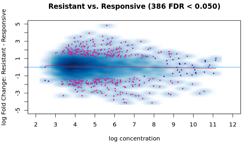
In my opinion, for visualization purposes it's accurate enough to convert the raw reads (bam files) to tdf format and load them in IGV with the option "normalize coverage data" enabled, this will rescale the raw counts to 1000000 / total counts.thus correcting for different library sizes. This assuming you are using/willing to use IGV, other browsers surely have similar options.
DiffBind, or rather the underlying edgeR and DESeq packages, don't make use of the read profiles. All they use are the raw counts of reads in given intervals (ChipSeq peaks, genes, whatever), in fact the read profile within an interval doesn't enter in the analysis at all.
If you want to show the log fold change you could prepare a bedgraph file where each line has as coordinates the region tested, or maybe the midpoint of the region tested, whichever looks better, and as value (4th column) the log fold change. Then load this file in IGV with or without the raw reads file as above.