Hello,

I was curious if anyone has any has any tips to identifying a composition vs. efficiency vs. trended bias in their data.

To preface this (because the users guide does cover this, and is helpful), our lab ran a ChIP-seq for H2AZ in three separate sequencing and IP batches. This is clearly evident on PCA as the samples cluster along dim1 primarily based on their batch identity rather than their genotype.

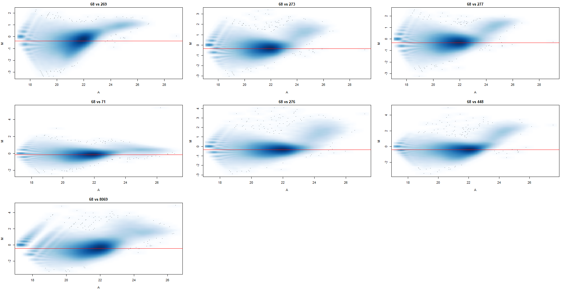
From our experience, we would expect a composition bias, and profile plots around the TSS and centered peaks corroborate this where we see a genotype-dependent accumulation of this histone variant, and so I began by normalizing for a composition bias. I tried a range of bin sizes (2k - 15k) as recommended by the users guide, and settled on 10k where the normalization factors weren't changing by much as I increased from there. I've attached the MA plots below, with norm.factors as follows

normFactors(Bins_Females_SampleFiltered_10k , se.out = F)$norm.factors
[1] 0.8136641 1.0391248 1.0248323 1.0111012 0.9129898 1.0366513 1.0851679 1.1113328

From this dataset, I've identified 2 outliers already through PCA and QC scores that have been removed (not in these MA plots). Based on the pattern of the clouds and the loess regression < 0 I would assume that there is in fact a composition bias, but what I find strange is that it's not really visible between the genotypes. i.e.: the first 3 plots are part of genotype A and the last 4 are part of genotype B, with another caveat being that sample 68 (genotype A) and 71 (genotype B) are part of one independent batch - could this be the reason that they all look different.

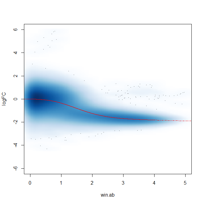
Additionally, after filtering windows and plotting abundance vs. FC plots, there appears to be a trended bias as well - though as far as I am aware this should be controlled for in the glmQLFit() portion of edgeR.

I was wondering if anyone has had issues with different sequencing batches similar to this and what they did to resolve them. I am getting the expected trend and number of DB sites and it lines up with our expectations of what's going on with this variant.

IIUC you're saying that 68 and 71 are more similar to each other than to all of the other replicates (more efficient IP, if I'm reading your plots correctly), and were generated in a separate sequencing + IP batch. This outcome seems pretty reasonable to me. I doubt that sequencing is the cause here but for some reason histone IP efficiency seems pretty sensitive to... everything, so can be expected to fluctuate between batches. (Can't remember if I ever figured out why this happens. TF ChIP-seq seems to be more stable between replicates, maybe there's less stuff happening at a binding site in open chromatin.)

Anyway, if you include the first IP batch as a blocking factor in your design matrix, the model should be able to naturally account for the differences between 68 + 71 versus all the other samples. This should manifest as a decrease in the dispersion because the model isn't being forced to consider the 68/71 as pure replicates of their corresponding genotypes.

Note that glmQLFit() will not account for the trended bias shown in these plots, the trend fitting in edgeR will only account for the mean-dispersion trend. If you want to remove the trended bias, you would need to generate and supply an offset matrix through the normOffsets() function. However, this assumes that the observed trend is actually bias and not genuine differences in binding between conditions. Given that you're normalizing for composition bias, you're already favoring the latter interpretation - which is fine, as long as you can justify it with external knowledge as you've described.