
Hello. I'm using edgeR to examine how gene expression changes in a control cell line vs. a genetically modified cell line at three timepoints. Each condition (ex. CTRL_DIV2, MOD_DIV2) has 3 replicates for a total of 18 samples.
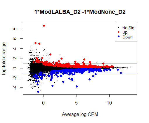
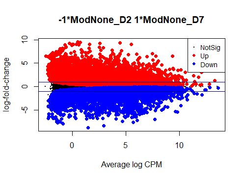
I see typical small DE gene ratios for contrasts between Mod - CTRL at the same timepoint, but a HUGE amount of DE genes (70 - 80%) in contrasts between different timepoints of the same cell line. Alongside timepoints, there are significant changes in cell culture conditions: D2 corresponds to 50% confluence, D4 100% confluence, and D7 is intentional overconfluence, glucose starvation and formation of complex structures.
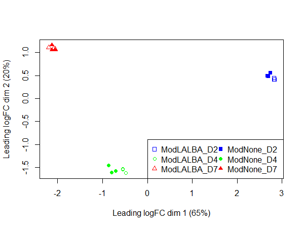
In the PCA plot, the replicates cluster well together and it appears most of the variation is explained by time in culture, consistent with the DE values.
Could anyone offer advice - could it be possible that this is biologically real?
EDIT: Cleaned up relevant code and including below:
## Prepare data files
fc <- readRDS("RNAseq.rds")
counts <- fc$counts
colnames(counts) <- sub("\\_.*", "", colnames(counts))
meta <- read.csv("metadata.csv")
meta <- meta[order(row.names(meta)),]
Group <- factor(paste0("Mod", meta$Mod, "_D", meta$DIV))
head(Group)
# [1] ModNone_D2  ModLALBA_D4 ModLALBA_D4 ModLALBA_D4 ModNone_D7
# [6] ModNone_D7
# 6 Levels: ModLALBA_D2 ModLALBA_D4 ModLALBA_D7 ... ModNone_D7

## Create DGElist
y <- DGEList(counts = counts,
             group = Group,
             lib.size = colSums(counts))
colnames(y) <- rownames(meta)


## Build and Ensembl-specific annotation lookup
mart <- useMart("ENSEMBL_MART_ENSEMBL")
mart <- useDataset("hsapiens_gene_ensembl", mart)
ens <- row.names(y)
ensLookup <- gsub("\\.[0-9]*$", "", ens)
head(ensLookup)

annotLookup <- getBM(
  mart=mart,
  attributes=c("ensembl_transcript_id", "ensembl_gene_id",
    "gene_biotype", "external_gene_name", "entrezgene_id"),
  filter="ensembl_gene_id",
  values=ensLookup,
  uniqueRows=TRUE)

annotLookup <- data.frame(
  ens[match(annotLookup$ensembl_gene_id, ensLookup)],
  annotLookup)
colnames(annotLookup) <- c("original_id", c("ensembl_transcript_id", "ensembl_gene_id", "gene_biotype", "external_gene_name", "entrezgene_id"))

summary(annotLookup)

 original_id        ensembl_transcript_id ensembl_gene_id
 Length:259537      Length:259537         Length:259537
 Class :character   Class :character      Class :character
 Mode  :character   Mode  :character      Mode  :character


 gene_biotype       external_gene_name entrezgene_id
 Length:259537      Length:259537      Min.   :        1
 Class :character   Class :character   1st Qu.:     7018
 Mode  :character   Mode  :character   Median :    51307
                                       Mean   : 12696013
                                       3rd Qu.:   146822
                                       Max.   :128966744
                                       NA's   :53659


## Annotation mapping
Symbol <- mapIds(org.Hs.eg.db,
                 keys=rownames(y),
                 keytype="ENSEMBL",
                 column="SYMBOL")

Symbol.df <- data.frame(Symbol=Symbol)
Symbol.df$ENTREZID <- annotLookup$entrezgene_id[match(Symbol.df$Symbol, annotLookup$external_gene_name)]
y$genes <- Symbol.df


## Filter genes and create design matrix
keep <- filterByExpr(y) # gene pool (including non-coding RNAs) size reduced from 62,696 --> 23,574
design <- model.matrix(~0 + Group)
colnames(design) <- levels(Group)
keep2 <- filterByExpr(y, design)
x <- y[keep2, , keep.lib.sizes = FALSE]
x <- calcNormFactors(x)


## Print MD plots in console (no QC issues detected)
#pdf(file = "MeanDifferencePlots.pdf")
#par(mfrow = c(3,3))
#for(i in 1:18){
#  print((plotMD(cpm(x, log=TRUE), column=i) + abline(h=0, col="red", lty=2, lwd=2)))
#}

points <- c(0,1,2,15,16,17)
colors <- rep(c("blue", "green", "red"), 2)
plotMDS(x, col=colors[Group], pch = points[Group])
legend("topleft", legend = levels(Group), pch = points, col = colors, ncol = 2)


# Estimate dispersion
x <- estimateDisp(x, design, robust = TRUE)
x$common.dispersion
# [1] 0.003289937

plotBCV(x)
saveRDS(x, file = "processed_data.rds")
x <- readRDS("processed_data.rds")


## Fit a GLM
fit <- glmQLFit(x, design, robust = TRUE)
QLDplot <- plotQLDisp(fit)


## Differential expression for one contrast (reference = edgeR manual section 4.4.8)
con1 <- makeContrasts(ModNone_D4 - ModNone_D2, levels=design)
qlf1 <- glmQLFTest(fit, contrast=con1)
summary(decideTests(qlf1, p.value = 0.05))
#       -1*ModNone_D2 1*ModNone_D4
#Down                         7687
#NotSig                       5743
#Up                           7906
#integer(0)

plotMD(qlf1) + abline(h = c(-1,1), col = "darkblue")

qlf1.df <- as.data.frame(qlf1)
EnhancedVolcano(qlf1.df,
                x = "logFC",
                y = "PValue",
                lab = qlf1.df$Symbol,
                FCcutoff = 1,
                pCutoff = 10e-6,
                title = "P2D11 NV DIV4 - P2D11 NV DIV2")


## Output tables for top DE genes and pathways
go <- goana(qlf1, species = "Hs", geneid = "ENTREZID")

topGOup <- topGO(go, ontology = "BP", sort = "up", n=100)
topGOdown <- topGO(go, ontology = "BP", sort = "down", n=100)

top1 <- as.data.frame(topTags(qlf1, n = 1000))
top1 <- top1[top1$FDR < 0.05,]
top1up <- top1[top1$logFC > 0,]
top1down <- top1[top1$logFC < 0,]


sessionInfo()
```
R version 4.2.2 (2022-10-31 ucrt)
Platform: x86_64-w64-mingw32/x64 (64-bit)
Running under: Windows 10 x64 (build 22631)

Matrix products: default

locale:
[1] LC_COLLATE=English_United States.utf8
[2] LC_CTYPE=English_United States.utf8
[3] LC_MONETARY=English_United States.utf8
[4] LC_NUMERIC=C
[5] LC_TIME=English_United States.utf8

attached base packages:
[1] stats4    stats     graphics  grDevices utils     datasets
[7] methods   base

other attached packages:
 [1] EnhancedVolcano_1.16.0 ggrepel_0.9.4
 [3] knitr_1.43             ggplot2_3.4.4
 [5] dplyr_1.1.2            plyr_1.8.8
 [7] openxlsx_4.2.5.2       GO.db_3.16.0
 [9] biomaRt_2.54.1         org.Hs.eg.db_3.16.0
[11] AnnotationDbi_1.60.2   IRanges_2.32.0
[13] S4Vectors_0.36.2       Biobase_2.58.0
[15] BiocGenerics_0.44.0    Rsubread_2.12.3
[17] edgeR_3.40.2           limma_3.54.2

loaded via a namespace (and not attached):
 [1] httr_1.4.7             splines_4.2.2
 [3] bit64_4.0.5            statmod_1.5.0
 [5] BiocManager_1.30.22    BiocFileCache_2.6.1
 [7] blob_1.2.4             GenomeInfoDbData_1.2.9
 [9] yaml_2.3.7             progress_1.2.2
[11] pillar_1.9.0           RSQLite_2.3.1
[13] lattice_0.20-45        glue_1.6.2
[15] digest_0.6.31          RColorBrewer_1.1-3
[17] XVector_0.38.0         colorspace_2.1-0
[19] htmltools_0.5.6        Matrix_1.6-1
[21] XML_3.99-0.14          pkgconfig_2.0.3
[23] zlibbioc_1.44.0        purrr_1.0.2
[25] scales_1.2.1           tibble_3.2.1
[27] KEGGREST_1.38.0        farver_2.1.1
[29] generics_0.1.3         cachem_1.0.8
[31] withr_2.5.0            cli_3.6.1
[33] magrittr_2.0.3         crayon_1.5.2
[35] memoise_2.0.1          evaluate_0.21
[37] fansi_1.0.4            xml2_1.3.5
[39] textshaping_0.3.6      tools_4.2.2
[41] prettyunits_1.1.1      hms_1.1.3
[43] lifecycle_1.0.3        stringr_1.5.0
[45] munsell_0.5.0          locfit_1.5-9.8
[47] zip_2.3.0              Biostrings_2.66.0
[49] compiler_4.2.2         GenomeInfoDb_1.34.9
[51] systemfonts_1.0.4      rlang_1.1.1
[53] grid_4.2.2             RCurl_1.98-1.12
[55] rstudioapi_0.15.0      rappdirs_0.3.3
[57] labeling_0.4.2         bitops_1.0-7
[59] rmarkdown_2.24         gtable_0.3.3
[61] DBI_1.1.3              curl_5.1.0
[63] R6_2.5.1               fastmap_1.1.1
[65] bit_4.0.5              utf8_1.2.3
[67] filelock_1.0.2         ragg_1.2.5
[69] stringi_1.7.12         Rcpp_1.0.11
[71] vctrs_0.6.3            png_0.1-8
[73] dbplyr_2.3.3           tidyselect_1.2.0
[75] xfun_0.40
```

Hi Gordon, thank you for replying! I've updated the original post to include code.
The NG dispersion is almost zero for your data, meaning that there is almost no biological variation between the replicates. There are also heaps of genes with very, very large fold-changes between the timepoints. So it's inevitable you'll get very large numbers of DE genes.
I'd recommend you use glmTreat() to reduce the number of DE genes before doing a GO analysis.
You might consider upgrading to the current version of Bioconductor, although it won't make much difference to your current analysis.