
Hi,
I compared raw count RNAseq data from 13 controls and 15 endometriosis lesions. The samples were not grouped by disease state as can be seen from the colData file:
disease_state
c1 control e1 endometriosis e2 endometriosis c2 control c3 control e3 endometriosis e4 endometriosis c4 control e5 endometriosis c5 control e6 endometriosis e7 endometriosis c6 control c7 control e8 endometriosis e9 endometriosis e10 endometriosis e11 endometriosis c8 control c9 control e12 endometriosis e13 endometriosis c10 control e14 endometriosis c11 control c12 control c13 control e15 endometriosis
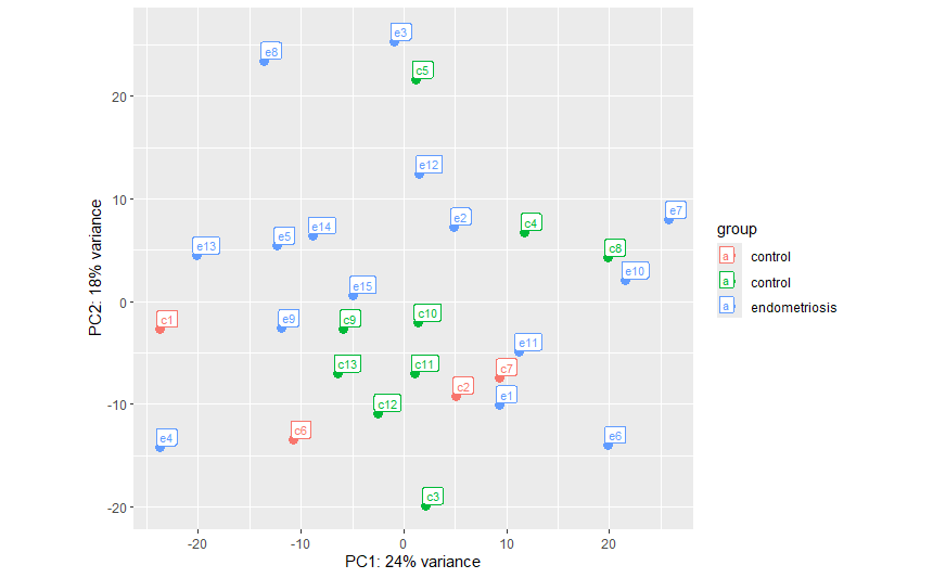
When I visualized the data with plotPCA from ggplot2 I noticed that the controls had been separated into 2 groups:
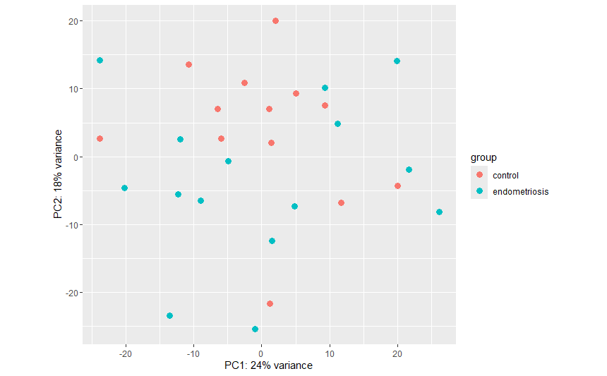
When I rearranged the order of the samples in the counts_data and colData files so that all of the controls were listed first and followed by the endometriosis samples, plotPCA gave a single control group and a endometriosis group as expected:
The DESeq2 output file was also different in these 2 analyses, even though the count data should be the same. Does anyone know what is going on here? Do I always need to keep the groups together in the input file?
Thanks for your help.
Code:
library(ggplot2)
library(tidyverse)

counts_data <- read.csv("C:\\Users\\Quanah\\ownCLoud\\PCOS_sub+visc_sequencing_data\\raw_counts_visc_endo_select.csv", header = TRUE, check.names = FALSE, row.names = 1)
colData <- read.csv("C:\\Users\\Quanah\\ownCLoud\\PCOS_sub+visc_sequencing_data\\sample_info_visc_endo_select.csv", header = TRUE, row.names = 1)

dds <- DESeqDataSetFromMatrix(countData = counts_data, colData = colData, design = ~ disease_state)

keep <- rowSums(counts(dds)) >= 10
dds <- dds[keep,]

dds$ disease_state <- relevel(dds$ disease_state, ref = "control")

dds <- DESeq(dds)

res <- results(dds)

res0.05 <- results(dds, alpha = 0.05)

plotMA(res0.05)

vsdata <-vst(dds, blind=FALSE)

plotPCA(vsdata, intgroup = "disease_state", ntop=500)

z <-plotPCA(vsdata, intgroup = "disease_state", ntop=500)

z + geom_label(aes(label = name),size = 3, hjust = 0.15, position = nudge)


sessionInfo( )
R version 4.3.3 (2024-02-29 ucrt) Platform: x86_64-w64-mingw32/x64 (64-bit) Running under: Windows 10 x64 (build 17763)
Matrix products: default
locale:
4 LC_COLLATE=English_Austria.1252 LC_CTYPE=English_Austria.1252
3 LC_MONETARY=English_Austria.1252 LC_NUMERIC=C
[5] LC_TIME=English_Austria.1252
time zone: Europe/Berlin tzcode source: internal
attached base packages: 4 stats4 stats graphics grDevices utils datasets methods base
other attached packages:
4 BiocManager_1.30.22 lubridate_1.9.3 forcats_1.0.0
4 stringr_1.5.1 dplyr_1.1.4 purrr_1.0.2
[7] readr_2.1.5 tidyr_1.3.1 tibble_3.2.1
[10] ggplot2_3.5.0 tidyverse_2.0.0 DESeq2_1.42.1
[13] SummarizedExperiment_1.32.0 Biobase_2.62.0 MatrixGenerics_1.14.0
[16] matrixStats_1.2.0 GenomicRanges_1.54.1 GenomeInfoDb_1.38.8
[19] IRanges_2.36.0 S4Vectors_0.40.2 BiocGenerics_0.48.1
loaded via a namespace (and not attached):
4 gtable_0.3.4 xfun_0.43 lattice_0.22-5
4 tzdb_0.4.0 vctrs_0.6.5 tools_4.3.3
[7] bitops_1.0-7 generics_0.1.3 parallel_4.3.3
[10] fansi_1.0.6 pkgconfig_2.0.3 Matrix_1.6-5
[13] lifecycle_1.0.4 GenomeInfoDbData_1.2.11 farver_2.1.1
[16] compiler_4.3.3 munsell_0.5.1 codetools_0.2-19
[19] htmltools_0.5.8.1 RCurl_1.98-1.14 pillar_1.9.0
[22] crayon_1.5.2 BiocParallel_1.36.0 DelayedArray_0.28.0
[25] abind_1.4-5 tidyselect_1.2.1 locfit_1.5-9.9
[28] digest_0.6.35 stringi_1.8.3 labeling_0.4.3
[31] fastmap_1.1.1 grid_4.3.3 colorspace_2.1-0
[34] cli_3.6.2 SparseArray_1.2.4 magrittr_2.0.3
[37] S4Arrays_1.2.1 utf8_1.2.4 withr_3.0.0
[40] scales_1.3.0 timechange_0.3.0 rmarkdown_2.26
[43] XVector_0.42.0 hms_1.1.3 evaluate_0.23
[46] knitr_1.46 rlang_1.1.3 Rcpp_1.0.12
[49] glue_1.7.0 rstudioapi_0.16.0 R6_2.5.1
[52] zlibbioc_1.48.2
