Question

Why is my plot count does not fit with log fold change result?

0

Entering edit mode

Gian ▴ 30

@chloe-25118

Last seen 2.3 years ago

Italy

Hi, I am new in R and I have performed DESEQ2 analysis and I am confused at a particular step

I try to plot the normalized counts into box plot but it does not match with the fold change results generated by Deseq2

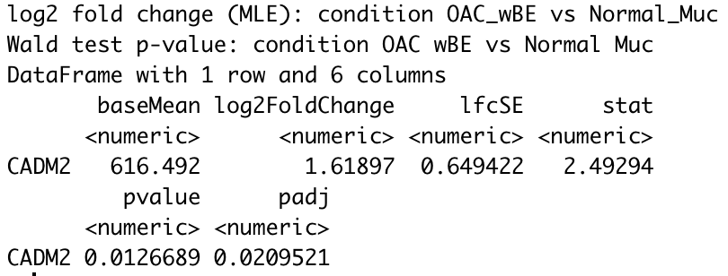
For instance, using CADM2 gene as an example and I compared OAC wBE with normal mucosa. The log2 fold change shows a positive 1.6 fold change higher in OAC wBE than normal mucosa.

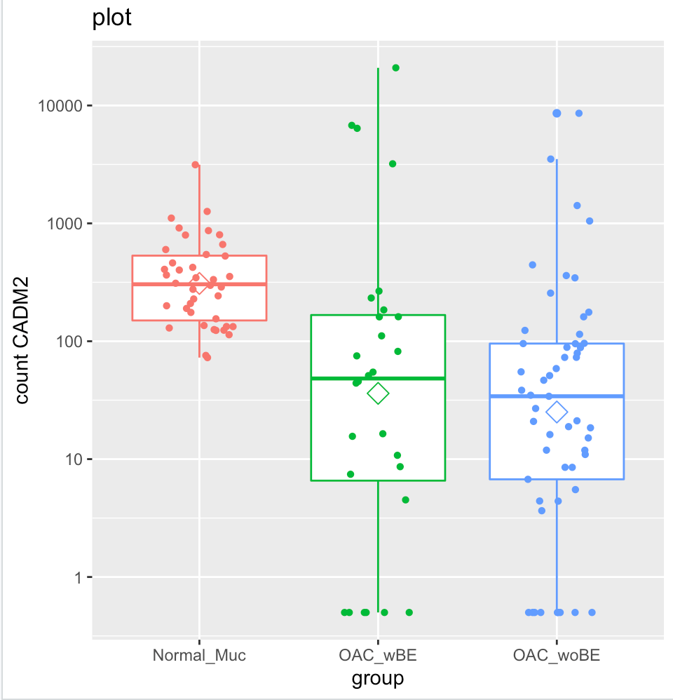
DESEQ2 result shows OAC_wBE has higher expression than Normal Muc

But when I plot them into a box plot, it shows that the normal mucosa has higher expression than OAC wBE. I have tried to extract the normalized counts of CADM2 and calculate the ratio of mean between the two groups, the result is similar with the log2foldchange result generated by DEseq2. However, when I plot it, the mean (shown in hexagonal white box) is higher in normal mucosa than OAC wBE. May I know, what is the problem here?

plot counts shows normal MUc has higher expression than OAC wBE

Here is the R code that I used

countsTable <- read.csv("merge_normal_cancer_5.csv",row.names = 1,sep=",")
summary(colSums(countsTable))
condition <- rep("Normal_Muc",121)
condition[which(grepl("woBE",names(countsTable)))] <- "OAC_woBE"
condition[which(grepl("wBE",names(countsTable)))] <- "OAC_wBE"
colours = c("darksalmon","lightblue2", "olivedrab2")
colData<-data.frame(condition,colours=colours[c(as.numeric(as.factor(condition)))])
row.names(colData)<-colnames(countsTable)
colData
colData$condition <- relevel(factor(colData$condition), ref = "Normal_Muc")

library(DESeq2)
dds<-DESeqDataSetFromMatrix(countData= countsTable,colData=colData,design=~condition)
dds<-DESeq(dds)
res <- results(dds)
head(results(dds, tidy=TRUE))
summary(res)
head(res)
head(dds)
View(dds)

normalized.counts <- as.data.frame(counts(dds, normalized=TRUE ))
write.csv(normalized.counts, "merge_normalized_counts.csv")

res_woBE_muc <- results(dds,contrast=c("condition","OAC_woBE","Normal_Muc"))
res_wBE_muc <- results(dds, contrast=c("condition", "OAC_wBE","Normal_Muc"))
res_woBE_wBE <- results(dds, contrast=c("condition", "OAC_woBE","OAC_wBE"))

write.csv(res_woBE_muc, "res_woBE_muc.csv")
write.csv(res_wBE_muc, "res_wBE_muc.csv")
write.csv(res_woBE_wBE, "res_woBE_wBE.csv")

res_woBE_muc <- res_woBE_muc[order(res_woBE_muc$padj),]
res_wBE_muc <- res_wBE_muc[order(res_wBE_muc$padj),]

rstudioapi::writeRStudioPreference("data_viewer_max_columns", 1000L)

res_woBE_muc["CRIP3",]
res_wBE_muc["CADM2",]
res_woBE_wBE["SPP1",]

ab <- plotCounts(dds, gene="SPP1", intgroup="condition", returnData=TRUE)
pq <- ggplot(ab,aes(x=condition, y=count, color=condition)) +geom_boxplot()
pq + geom_jitter(shape=16, position=position_jitter(0.2)) + labs(title="plot",x="group", y="count SPP1")+scale_y_continuous(trans='log10')+stat_summary(fun.y=mean,geom="point",shape=23, size=4) 


# include your problematic code here with any corresponding output 
# please also include the results of running the following in an R session 

sessionInfo( )

DESeq2 • 2.0k views

ADD COMMENT • link updated 3.5 years ago by Michael Love 42k • written 3.5 years ago by Gian ▴ 30

score 0 · Answer 1 · 2021-06-08

0

Entering edit mode

Michael Love 42k

@mikelove

Last seen 3 hours ago

United States

Are you certain that you are plotting CADM2? The code says gene=SPP1.

What is:

mean(counts(dds, normalized=TRUE)["CADM2",dds$condition == "Normal_Muc"])
mean(counts(dds, normalized=TRUE)["CADM2",dds$condition == "OAC_wBE"])

Edit: Oh I see you said that you get the same LFC when you calculate it manually. This is because you have three samples with a very large count which is influencing the mean for OAC group. The ggplot2 is showing the mean of log counts, instead of the mean of the counts. I think your data is not actually Negative Binomial distributed within this group, but that there is remaining variation that gives you actually bimodal distribution within a group that should not be bimodal according to the model. Do you have unaccounted for batch effects? What does a PCA plot look like? It could be resolved with some batch effect modeling.

ADD COMMENT • link 3.5 years ago Michael Love 42k

0

Entering edit mode

Thank you Michael for your feedback.

Sorry, I was working at other gene which is SPP1, but I am sure the result was CADM2

To answer your question, I ran the code in R and I got:

mean(counts(dds, normalized=TRUE)["CADM2",dds$condition == "Normal_Muc"]) 1 451.0865 mean(counts(dds, normalized=TRUE)["CADM2",dds$condition == "OAC_wBE"]) 1 1385.802

I ran this code to obtain the PCA plot vsd <- vst(dds, blind=FALSE)

library("RColorBrewer") library(pheatmap) sampleDists <- dist(t(assay(vsd))) sampleDistMatrix <- as.matrix(sampleDists) rownames(sampleDistMatrix) <- paste(vsd$condition, vsd$type, sep="-") colnames(sampleDistMatrix) <- NULL colors <- colorRampPalette( rev(brewer.pal(9, "Blues")) )(255) pheatmap(sampleDistMatrix, clustering_distance_rows=sampleDists, clustering_distance_cols=sampleDists, col=colors)

plotPCA(vsd, intgroup=c("condition")) coord_fixed()

PCA plot

Unfortunately, I do not have any information regarding the which do these samples come from. How will I be able to account for batch effects? Thank you

ADD REPLY • link 3.5 years ago Gian ▴ 30

0

Entering edit mode

I think you have batch-like variation within the OAC groups and it would be better to control for it in the design. You can do SVA or RUV (pick one of these) and then add the SV or FUV to the design as variables to control:

http://master.bioconductor.org/packages/release/workflows/vignettes/rnaseqGene/inst/doc/rnaseqGene.html#removing-hidden-batch-effects

ADD REPLY • link 3.5 years ago Michael Love 42k

0

Entering edit mode

Thank you Michael for your feedback

I have done RUVSeq according to your recommendation and re-run DEseq afterwards. However, I still get the same graphs where the normal mucosa is higher in the plotcount while OACwBE is lower. On the other hand, the foldchange has increased dramatically.

I do apologize beforehand that I am still a beginner in using R. Thank you

enter image description here

## setting RUVSeq  
  BiocManager::install("RUVSeq")
  library("RUVSeq")  

  set <- newSeqExpressionSet(counts(dds))
  idx  <- rowSums(counts(set) > 5) >= 2
  set  <- set[idx, ]
  set <- betweenLaneNormalization(set, which="upper")
  not.sig <- rownames(res)[which(res$pvalue > .1)]
  empirical <- rownames(set)[ rownames(set) %in% not.sig ]
  set <- RUVg(set, empirical, k=2)
  pData(set)

## rerun DESEQ using RUVSeq  
  ddsruv <- dds
  ddsruv$W1 <- set$W_1
  ddsruv$W2 <- set$W_2
  design(ddsruv) <- ~ W1 + W2 + condition

dds<-DESeq(ddsruv)
res <- results(dds)
head(results(dds, tidy=TRUE))
summary(res)
head(res)
head(dds)

res_woBE_muc <- results(dds,contrast=c("condition","OAC_woBE","Normal_Muc"))
res_wBE_muc <- results(dds, contrast=c("condition", "OAC_wBE","Normal_Muc"))
res_woBE_wBE <- results(dds, contrast=c("condition", "OAC_woBE","OAC_wBE"))

res_woBE_muc["CRIP3",]
res_wBE_muc["CADM2",]
res_woBE_wBE["SPP1",]

ab <- plotCounts(dds, gene="CADM2", intgroup="condition", returnData=TRUE)
pq <- ggplot(ab,aes(x=condition, y=count, color=condition)) +geom_boxplot()
pq + geom_jitter(shape=16, position=position_jitter(0.2)) + labs(title="plot",x="group", y="count CADM2")+scale_y_continuous(trans='log10')+stat_summary(fun.y=mean,geom="point",shape=23, size=4)

ADD REPLY • link 3.5 years ago Gian ▴ 30

0

Entering edit mode

The plot will not change (it just shows counts scaled for sequencing depth), but now the results take into account variation within your groups. This can change results in either direction, genes can become less significant or more significant, depending on how the nuisance variation correlates with your condition of interest.

I think this is a difficult gene to assess, as some of the samples are up-regulated and some are down-regulated with respect to the control group. You have a heterogeneous response relative to the control group.

Can you assess if the samples with high counts for this gene are also outliers in the PCA plot and the plot of W1 vs W2? If so, you may want to do a sensitivity analysis where you remove these dozen or so samples and re-run DESeq2. You could then consider to prioritize genes that do not lose significance when those samples are removed.

ADD REPLY • link 3.5 years ago Michael Love 42k

0

Entering edit mode

Thank you for your reply Michael,

Actually, I am not particularly looking at this gene. Instead, I am actually selecting highly differentially expressed genes based on large baseMean to perform Immunohistochemistry. Because I am selecting large baseMean, this issue keeps occuring to other genes. Therefore, I can not select which samples that has high counts for this particular genes to remove the samples as I have to take into account for other genes as well.

As you mentioned earlier that as there are huge counts that affect the mean of my OAC group. Is it suitable to calculate the ratio of median of these genes from the normalized value instead of calculating the ratio of the mean? Then, I will calculate the p value manually by using Mann-Whitney?

ADD REPLY • link 3.5 years ago Gian ▴ 30

0

Entering edit mode

Still if I were you I would explore the relationship between the high counts for this particular gene (and others like it) and the outliers in the PCA / RUV scatterplot (that is just for attempting to understand what is going on). I often find that going back and forth between individual gene plots and systematic plots helps me understand what is happening.

But whether you do that or not, I would still recommend to remove the outlier samples in both OAC groups and re-run DESeq() to see which genes remain significant.

Or, alternatively, for non-parametric testing, you could use one of the methods already designed for RNA-seq: SAMseq (if you have counts only) or Swish (from my group, designed for use with Salmon quantification data).

SAMseq is simple to try:

library(SAMseq)
keep <- rowSums(counts(dds) >= 10) >= N
x <- counts(dds)[keep,]
y <- dds$condition
fit <- SAMseq(x=x, y=y, resp.type="Two class unpaired", fdr.output=0.1)
head(fit$siggenes.table$genes.up)
head(fit$siggenes.table$genes.lo)

ADD REPLY • link 3.5 years ago Michael Love 42k

0

Entering edit mode

Thank you for your reply Michael,

I am performing the SAMseq but it is taking so long to run ( I think it has been running for 2 hours). I hope this is normal occurence. I am also looking back at my PCA/ RUV scatter plot and notice there are some samples that are out of their group. In case I remove them, how will I be able to know that these samples are not essential in my analysis?

Also, I realize that this situation occurs because I am comparing my cancer samples from TCGA (OAC wBE & OAC woBE) with normal sample that I obtain from GTEx. When I perform DESeq analysis to compare between only these two cancers I obtained from TCGA, there are not much issue. Is it possible that this issue occur because I am trying to compare these cancer samples to normal samples from GTEx?

my PCA plot and distance heatmap without normal looks like this:

enter image description here

Is it safe for me to say that I can normally perform DEseq2 on OAC woBE and wBE. But, the problem arise because I am comparing with normal tissue from other database which may cause batch bias?

ADD REPLY • link 3.5 years ago Gian ▴ 30

0

Entering edit mode

"In case I remove them, how will I be able to know that these samples are not essential in my analysis?"

I'm suggesting the opposite, as a sensitivity analysis: what if these outliers are driving the differences.

In the end these decisions are up to you as the analyst. I can provide pointers on why results happen (e.g. because you are comparing mean expression, not log of mean expression here), but you'll have to make the analysis choices.

ADD REPLY • link 3.5 years ago Michael Love 42k