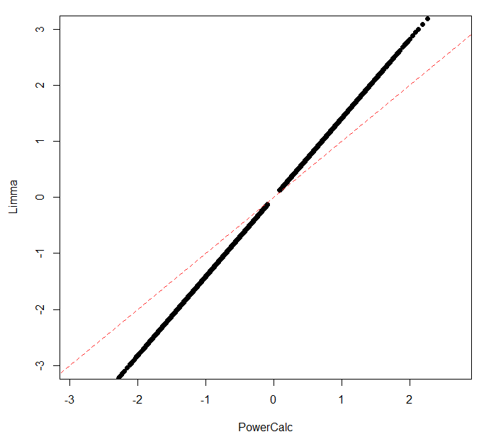
I am currently working on Illumina HumanMethylation Array (EPIC and HM450K) data. I wanted to do some power calculations for a dataset that consists of paired data. First, I calculated the effect size using Cohens D formula for paired data (found here). Later, I wanted to check how the power is affected when I use the effect size calculated with the shrunken variance from the eBayes function (fit$s2.post) in LIMMA as recommended here. As expected, I found that the eBayes estimate s2.post yielded greater effect sizes compared to the standard method. Interestingly, however, when I used the ordinary standard deviation from the LIMMA analysis, I also get larger effect sizes for CpG probes in general (see table and figure below). I did not expect the results to be exactly the same, but it still made me question my approach. Is there something wrong or is this difference to be expected?
Best regards
Table:
            ES(myFunc)     ES(s2.post)  ES(sigma)
cg11527153  0.6650809      0.9842229    0.9405664
cg27573606 -0.7264109     -0.7207224   -1.0273001
cg08128007 -0.6761195     -1.0389345   -0.9561774
cg04407431 -0.7193812     -0.9974031   -1.0173586
cg08900511  0.5606958      0.8301470    0.7929436
cg06623778 -0.4489218     -0.6930386   -0.6348712
cg17436295 -0.6082728     -0.8160284   -0.8602276
cg13176867 -0.4855485     -0.7544834   -0.6866693
cg15105996 -0.6920180     -1.0432545   -0.9786612
cg09856436 -0.6109584     -0.9215909   -0.8640257
ES(myFunc) = mean(pairwise difference)/SD(pairwise difference); (more details in code below)
ES(s2.post) = (fit2_D1$coefficients / sqrt(fit2_D1$s2.post))
ES(sigma) = (fit2_D1$coefficients / (fit2_D1$sigma))
Figure:
Note: Difference in effect size calculate by LIMMA (using fit2_D1$sigma) and my function (see Snippet "cohensD_Paired"). Dotted line : y = x. I removed probes with effect size below |0.1| as I got errors during power calculation as the sample size estimates were too big.
Snippet from my code used for power calculation
# Effect Size for power calculation

# split M-value Matrix by Groups (nameGroups corresponds to Sample_Group in the Limma analysis)
M1 <- beta[,which(pdGroups == nameGroups[1])]
M2 <- beta[,which(pdGroups == nameGroups[2])]

# Order samples accoding to pairs for subsequent subtraction
M1 <- M1[,order(colnames(M1))]
M2 <- M2[,order(colnames(M2))]

# Calculate difference of pairs
D <- M2 - M1

# mean of difference
meanD <- rowMeans(D)

# sigma of difference
sigmaD <- sqrt(matrixStats::rowVars(D))

# calculate CohensD
CohensD <- cohensD_Paired(meanD = meanD,
                          sigmaD = sigmaD)

# Function used above
# cohensD_Paired <- function(meanD, sigmaD){
#   return(meanD/sigmaD)}
Snippet from my code used for limma
# Effect Size of paired analysis in Limma

# Paired Design Matrix
design1 <- model.matrix(~ 0 + Sample_Group + Pair, data = pdLimma)

# M-Value Matrix
fit_D1 <- lmFit(Beta_To_M(betaMatrix), design1)

# Group Contrast
contMatrix_D1 <- makeContrasts(Sample_GroupPrimary-Sample_GroupMet ,levels=design1)
fit2_D1 <- contrasts.fit(fit_D1, contMatrix_D1)

# Ebayes
fit2_D1 <- eBayes(fit2_D1)

# Effect size (sigma)
(fit2_D1$coefficients / (fit2_D1$sigma))

# Effect size (eBayes)
(fit2_D1$coefficients / sqrt(fit2_D1$s2.post))
Session Info
R version 4.0.3 (2020-10-10)
Platform: x86_64-w64-mingw32/x64 (64-bit)
Running under: Windows 10 x64 (build 18363)

Matrix products: default

locale:
[1] LC_COLLATE=German_Switzerland.1252  LC_CTYPE=German_Switzerland.1252
[3] LC_MONETARY=German_Switzerland.1252 LC_NUMERIC=C
[5] LC_TIME=German_Switzerland.1252

attached base packages:
[1] stats     graphics  grDevices utils     datasets  methods   base

other attached packages:
[1] ggplot2_3.3.2 limma_3.44.3

loaded via a namespace (and not attached):
 [1] rstudioapi_0.13     magrittr_2.0.1      BiocGenerics_0.35.4 tidyselect_1.1.0    munsell_0.5.0
 [6] lattice_0.20-41     viridisLite_0.3.0   colorspace_2.0-0    R6_2.5.0            rlang_0.4.9
[11] dplyr_1.0.2         tools_4.0.3         parallel_4.0.3      grid_4.0.3          gtable_0.3.0
[16] withr_2.3.0         ellipsis_0.3.1      matrixStats_0.57.0  digest_0.6.27       tibble_3.0.4
[21] lifecycle_0.2.0     crayon_1.3.4        farver_2.0.3        purrr_0.3.4         vctrs_0.3.6
[26] S4Vectors_0.26.1    glue_1.4.2          labeling_0.4.2      compiler_4.0.3      pillar_1.4.7
[31] generics_0.1.0      scales_1.1.1        stats4_4.0.3        hexbin_1.28.1       pkgconfig_2.0.3   R version 4.0.3 (2020-10-10)
Platform: x86_64-w64-mingw32/x64 (64-bit)
Running under: Windows 10 x64 (build 18363)

Matrix products: default

locale:
[1] LC_COLLATE=German_Switzerland.1252  LC_CTYPE=German_Switzerland.1252
[3] LC_MONETARY=German_Switzerland.1252 LC_NUMERIC=C
[5] LC_TIME=German_Switzerland.1252

attached base packages:
[1] stats     graphics  grDevices utils     datasets  methods   base

other attached packages:
[1] ggplot2_3.3.2 limma_3.44.3

loaded via a namespace (and not attached):
 [1] rstudioapi_0.13     magrittr_2.0.1      BiocGenerics_0.35.4 tidyselect_1.1.0    munsell_0.5.0
 [6] lattice_0.20-41     viridisLite_0.3.0   colorspace_2.0-0    R6_2.5.0            rlang_0.4.9
[11] dplyr_1.0.2         tools_4.0.3         parallel_4.0.3      grid_4.0.3          gtable_0.3.0
[16] withr_2.3.0         ellipsis_0.3.1      matrixStats_0.57.0  digest_0.6.27       tibble_3.0.4
[21] lifecycle_0.2.0     crayon_1.3.4        farver_2.0.3        purrr_0.3.4         vctrs_0.3.6
[26] S4Vectors_0.26.1    glue_1.4.2          labeling_0.4.2      compiler_4.0.3      pillar_1.4.7
[31] generics_0.1.0      scales_1.1.1        stats4_4.0.3        hexbin_1.28.1       pkgconfig_2.0.3


Thank you very much for the clarification! My thinking was that using
sigmaands2.postas mentioned above would also describe the difference between two observations since I use a contrast matrix that specifies the difference between group1 and group2, which also encompasses the difference of the pairs. But I see now that this was a misconception. I m intrigued about the sqrt(2). Why is multiplying the residual standard deviation (sqrt(sum(Y-Y_hat)^2/n-p)) by sqrt(2) equal to the standard deviation of a difference of two observations (sqrt(sum((G2-G1)-mean(G2-G1))^2/n))?It's just undergrad stats. var(X1-X2) = var(X1)+var(X2) = $\sigma^2 + \sigma^2 = 2\sigma^2$.